Constrained K-means Clustering for Stratification
I’ve been learning a lot about randomization over the past few weeks. Specifically, I have been reading up on the benefits of matched-pair designs over basic randomization. Bai (2020a, 2020b), Athey and Imbens (2016), and Imai et al. (2020), each provide theoretical and practical insights into the benefits of matched-pair randomization, where, in a simple treatment-control design, the researcher creates pairs of units at the level of randomization based on some baseline characteristic (e.g. income, population, geographic size, proximity, etc.), and then randomly assigns one of the pairs into the treatment, and the other into the control.
My curiosity was piqued when I tried to find papers that used matched-pairs for a multi-arm experiment, that is, an experiment with more than one treatment (or control) group. Lu et al. (2011), Lu and Rosenbaum (2004), and Greevy (2004) talk about optimal nonbipartite matching (which sounds very fancy) but only consider instances with three treatment arms. Having just worked on a project with five arms, I was interested to see if any work focused on quinquepartite matching, and quickly realized that no such work existed. Realizing also that quinquepartite matching was a ridiculous prospect, I think set about thinking of ways to do something similar. I had in mind a sort of clustering and stratification method that grouped similar units together, and then randomly assigned the different treatment groups within those clusters.
And so began my adventure into constrained k-means clustering…
Having conducted a brief review on clustering and stratification methods for randomization, I realized that what I was looking for was a function that grouped similar units together. K-means seemed like a solid candidate to do so. However, k-means clustering algorithms don’t like to have a size constraint on them. They prefer to split the data into groups based on characteristics, not based on quotas. This was my first challenge, figuring out whether it was statistically legal to put a cluster size constraint on a k-means algorithm and whether I could figure out a way to do this in R.
The second challenge arose during a discussion with the PIs at PGRP. Say we were creating groups of units based on geographical proximity and population size. We would be matching on three variables, the latitude, longitude, and population number. If these covariates were all equally weighted, we wouldn’t reap the logistical benefits of keeping the units close together, as the population variable might cause the algorithm to match units that end up being pretty far away. We also have reason to believe that geographically proximate units are more likely to be similar on other baseline characteristics. The problem then becomes coming up with a good way to weight the covariates on which we are clustering. This problem will be addressed as a separate article at a later date…
After a good deal of having no idea of what was going on, several discussions with my co-workers, and literally days of stackoverflow digging, I arrived at a solution.
First, let’s get set up:
library(magrittr)## Warning: package 'magrittr' was built under R version 4.2.3library(ggplot2)## Warning: package 'ggplot2' was built under R version 4.2.3Now, let’s generate some datums:
# Set seed for reproducibility
set.seed(1234)

dat <-
  expand.grid(
    district         = c(1:2),
    sub_district     = c(1:7),
    sub_sub_district = c(1:19),
    village_id       = c(1:2)
  ) %>%
  dplyr::group_by(district, sub_district, sub_sub_district, village_id) %>%
  dplyr::mutate(
    # Total population
    tot_pop = rnorm(n = 1, mean = 100, sd = 5000),
    # Number of primary schools
    p_schl = rnorm(n = 1, mean = 2, sd = 6),
    # Paved road
    p_road = sample(0:1, size = dplyr::row_number(), replace = FALSE)
  ) %>%
  dplyr::group_by(district, sub_district, sub_sub_district, village_id) %>%
  dplyr::mutate(
    # Size of village in hectares
    town_hec = rnorm(n = 1, mean = 300, sd = 320)
  ) %>%
  dplyr::group_by(district, sub_district, sub_sub_district, village_id) %>%
  dplyr::mutate(
    # Coordinates
    x_cent = rnorm(n = 1, mean = 99.9, sd = 0.66),
    y_cent = rnorm(n = 1, mean = 33.3, sd = 0.33)
  ) %>%
  dplyr::ungroup()
Let’s look at dat:
dat## # A tibble: 532 × 10
## district sub_district sub_sub_district village_id tot_pop p_schl p_road
## <int> <int> <int> <int> <dbl> <dbl> <int>
## 1 1 1 1 1 -5935. 0.361 1
## 2 2 1 1 1 -1093. -5.50 1
## 3 1 2 1 1 -1371. 0.663 0
## 4 2 2 1 1 218. 15.5 1
## 5 1 3 1 1 -6854. -4.88 1
## 6 2 3 1 1 4877. -7.11 0
## 7 1 4 1 1 212. 1.31 1
## 8 2 4 1 1 -9075. 6.04 0
## 9 1 5 1 1 8294. -4.69 1
## 10 2 5 1 1 2888. -2.48 1
## # ℹ 522 more rows
## # ℹ 3 more variables: town_hec <dbl>, x_cent <dbl>, y_cent <dbl>dat looks good.
Now, above I mentioned that the whole “figuring out a way to apply econometrically sensible/not totally arbitrary weights to our covariates” conundrum would be tackled in a later article, so for the time being, we can be very arbitrary in how we apply weights. In any case, we want to apply a larger weight to the spatial variables as we believe that spatial covariates are more important than aspatial ones when it comes to clustering. Below, we see that the latitude and longitude are weighted 10:1 with the population variable.
dat <-
  dplyr::mutate(
    dat,
    x_cent = scales::rescale(x_cent, to = c(0, 10)),
    y_cent = scales::rescale(y_cent, to = c(0, 10)),
    tot_pop = scales::rescale(tot_pop, to = c(0, 1))
    )
Hierarchical clustering—the fancy word for what we are doing right now—algorithms require a distance matrix to generate the right clusters. That means we need to subset our entire dataset to only the variables that we want to compute distances for, i.e., the three variables above.
# Subset
dat <- dplyr::select(dat, x_cent, y_cent, tot_pop)

# Calculate distances
dist <- distances::distances(as.data.frame(dat))
Now comes the cool bit. I think this next segment is made even cooler because I don’t think there’s ever been a time when I’ve had an issue, searched for the solution, and found a package that does exactly what I wanted it to do in literally one line of code. The whole experience felt too good to be true (maybe it is – please email me if you see me making any statistically illegal claims. Thanks.).
The package scclust—size-constrained clustering—does exactly what it says on the CRAN tin. In baby terms, it just takes a k-means algorithm and puts a size constraint on it. Given that I have been talking about studies with five treatment arms, I put a size constraint of 5 below.
clust <- scclust::hierarchical_clustering(distances = dist, size_constraint = 5)Magical. Now let’s clean up our datasets by joining clust with dat.
final <-
  dplyr::bind_cols(dat, clust) %>%
  dplyr::rename(block = `...4`)
## New names:
## • `` -> `...4`Let’s have a quick peek at the output to make sure it’s doing what we hope it’s doing:
investigate_cluster <-
  dplyr::group_by(final, block) %>%
  dplyr::summarise(count = length(block))

investigate_cluster
## # A tibble: 106 × 2
## block count
## <scclust> <int>
## 1 0 5
## 2 1 5
## 3 2 5
## 4 3 5
## 5 4 5
## 6 5 5
## 7 6 5
## 8 7 5
## 9 8 5
## 10 9 5
## # ℹ 96 more rowsLooks good. It looks like each block is of size 5. Let’s double check:
max(investigate_cluster$count)## [1] 7table(investigate_cluster$count)##
## 5 7
## 105 1Interesting, looks like they’re not equal. So, because dat contains 532 observations (which, if my limited mathematical knowledge pays off, is not divisible by five), the algorithm automatically creates a sort of “overflow” group. Neat. This isn’t super convenient in my case, so I will add an extra section on how to alter this default.
Anyway, let’s now visualize the algorithm on our dummy data. I use the nifty package ggConvexHull to visualize the clusters.
ggplot(
  final,
  mapping = aes(
    x = x_cent,
    y = y_cent,
    color = factor(block)
    )
  ) +
  geom_point() +
  ggConvexHull::geom_convexhull(
    alpha = .5,
    aes(
      fill = factor(block)
      )
    ) +
  theme_bw() +
  theme(legend.position = "none")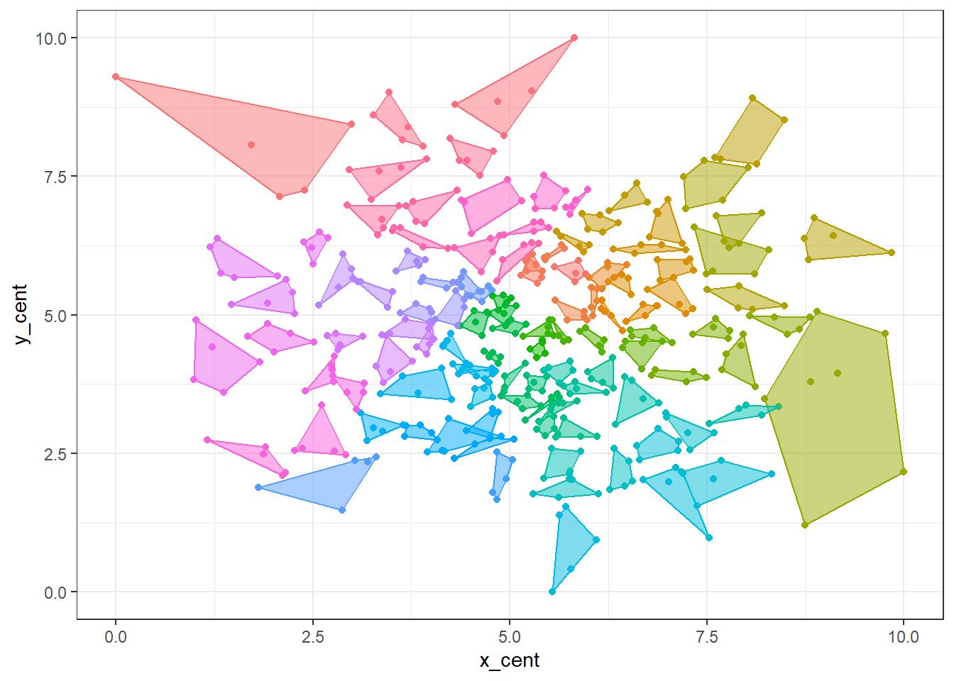
We can see that the points have been grouped in fives, except for that one cluster in the bottom right-hand corner. Notice how that cluster of seven has another cluster protruding into it – had we not included tot_pop in the distance matrix, each cluster would be entirely spatially distinct as we would clustering solely based on location.
So that is how we can create clusters based on spatial and aspatial covariates.
Extra stuff
I don’t like that pesky group of seven. I would rather create an overflow group of two, and keep those as spare units in case we need them. I will run through the procedure in-line below:
# Define number of treatment waves
number_of_waves <- 5

# REPRODUCIBILITY!!!
set.seed(1234)

final_treated <-
  final %>%
  dplyr::arrange(block) %>%
  dplyr::group_by(block) %>%

  # 1. Find the number of observations in each block
  dplyr::mutate(block_count = dplyr::row_number()) %>%
  dplyr::ungroup() %>%

  # 2. Create overflow group by setting block cutoff == number_of_waves
  dplyr::mutate(
    block = ifelse(
      block_count > number_of_waves,
      max(block) + 1,
      block
    )
  ) %>%

  # 3. Re-calculate block_count
  dplyr::group_by(block) %>%
  dplyr::mutate(block_count = max(dplyr::row_number())) %>%

  # 4. Apply treatment status
  dplyr::mutate(
    treatment = ifelse(
      block_count == number_of_waves,
      sample(c(number_of_waves), dplyr::n(), replace = FALSE),
      sample(sample(number_of_waves, max(block_count)), dplyr::n(), replace = FALSE)
    )
  )
Point 4. needs some extra explanation. For clusters that have exactly five units with them are randomly assigned one of the five treatment waves or phases. Then, for clusters that do not contain the exact number of waves—e.g. that cluster of two observations—we randomly assign them to any of the five waves.
Let’s visualize it.
# Plot results
treated_visual <-
  ggplot() +
  geom_point(
    final_treated,
    mapping = aes(
      x = x_cent,
      y = y_cent,
      color = factor(treatment)
      ),
    size = 1
    ) +
  ggConvexHull::geom_convexhull(
    final_treated,
    alpha = .5,
    mapping = aes(
      x = x_cent,
      y = y_cent,
      fill = factor(block)
      )
    ) +
  scale_fill_manual(
    values = rep("grey", length(unique(final_treated$block)))
    ) +
  scale_color_manual(
    values = c("1" = "dodgerblue4", "2" = "turquoise4", "3" = "red4", "4" = "orange2", "5" = "yellow3")
    ) +
  labs(
    x = "",
    y = "",
    color = "Treatment group"
    ) +
  guides(fill = FALSE) +
  theme_bw()
## Warning: The `<scale>` argument of `guides()` cannot be `FALSE`. Use "none" instead as
## of ggplot2 3.3.4.
## This warning is displayed once every 8 hours.
## Call `lifecycle::last_lifecycle_warnings()` to see where this warning was
## generated.treated_visual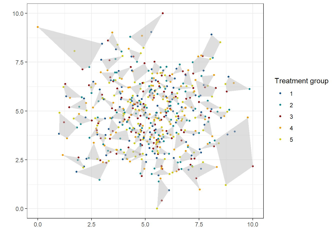
That concludes today’s post. This will lead us nicely into the next ridiculously niche plot post, which will give an overview of calculating optimal euclidean distances between units within a cluster. Stay tuned!